Visualizing transformations

The bottom group of buttons on the right are for actually visualizing transformations. This is the crux of the app.

The reset button simply resets the position of the basis vectors to the identity. It does not reset the zoom level, display settings, or polygon. These are done separately.

The text box along the bottom is the expression input box, which is where your expressions go when you want to visualize them. You can then use the up and down arrow keys to scroll through previously used expressions.

Render

When rendering an expression, the app will evaluate whatever expression you’ve typed into the expression input box, and just render it in the viewport. This means it will put the \(i\) vector at the position specified by the first column, and the \(j\) vector at the position specified by the second.

If you render the same expression twice in a row, then it will be exactly the same as just rendering it once.

Animate

The animate button does exactly as it says - it animates. However, there are two distinct types of animation - Transitive and Applicative. The default is Applicative, but you can change it in the display settings.

Animation also supports the use of commas to separate expressions. Each expression between commas must be valid on its own. These expressions will be animated one-by-one, going from left to right.

Transitive

Transitive animation is the simplest form. It’s basically just rendering, but instead of the basis vectors jumping to their new positions, they get dragged there and you can watch them move.

If you animate the same expression twice with Transitive animation, the first time will look like an animation, but the second time will look like nothing happens. This is because each point gets dragged to its new position, which is exactly the same as its current position, so nothing actually moves.

Applicative

Applicative animation is much more interesting, and is one of the reasons I decided to make lintrans in the first place.

Let’s define a matrix \(\mathbf{C}\) to represent whatever is currently being displayed in the viewport. If the result of evaluating the expression input box is a matrix \(\mathbf{E}\), and we want to render a target matrix \(\mathbf{T}\), then \(\mathbf{T} = \mathbf{EC}\).

Intuitively, Applicative animation takes the transformation represented by the given expression and applies it to the current state of the viewport, hence the name.

If you animate the same matrix A twice with Applicative animation, then the end result will be the same as rendering A^2, IF you started from the identity. If start by rendering a matrix B, and then animate A twice, then you’ll end up with what you would get if you just rendered A^2B.

With Applicative animation, commas do not affect the final result. They just show you the steps taken to get there. But when using commas with Transitive animation, the result is the same as just rendering the expression on the left.

The examples below (using Applicative animation and the matrix \(\mathbf{B}\) from defining matrices visually) show that the order of matrices in the expression changes the result of animation. This is because matrix multiplication is non-commutative.

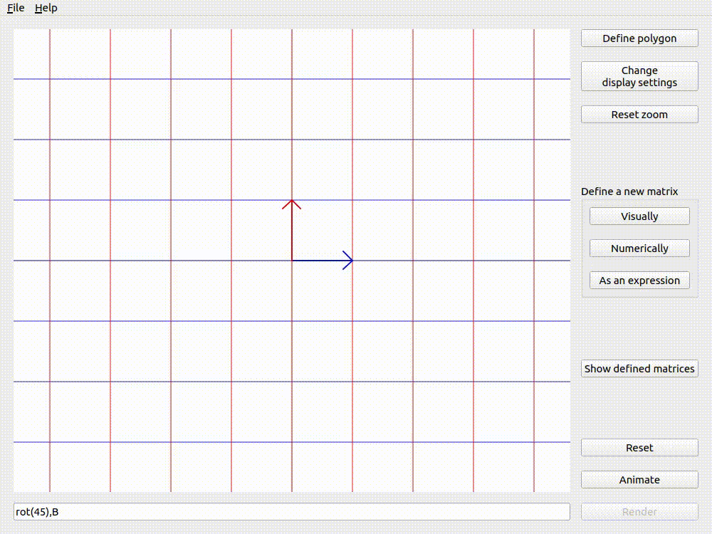
Animating rot(45),B with Applicative animation

Animating B,rot(45) with Applicative animation

Using input and output vectors

It is often helpful to imagine a single point and how it would get transformed by a given transformation. lintrans provides an input vector that you can drag around the viewport, and see the associated output vector - the input vector transformed by the matrix.

It is useful to drag this input vector around and see where it lines up with the output vector. This is helpful for finding invariant lines. You can then enable eigenlines to see where these invariant lines actually are, and the eigenvectors will let you see the scale factors associated with these lines. See the display setting linked previously for details.

It is also useful to have an input vector in the viewport and ask your students to find its image under the displayed transformation. It is easy to verify their answers by just displaying the output vector.

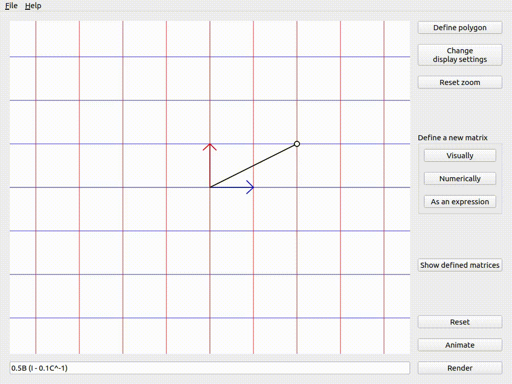
The input and output vectors shown for 0.5B (I - 0.1C^-1)

Defining custom polygons

It is often useful to think about a shape and how it would get transformed by a given matrix. lintrans allows you to define a polygon using the Define polygon button. Clicking it will open a dialog box where you can click to add as many vertices to the polygon as you would like. You can drag vertices around, they will snap to integer coordinates, and you can delete vertices by right clicking on them.

You can then see this polygon before and after the transformation when you render or animate an expression. The before and after versions can be independently hidden in the display settings.

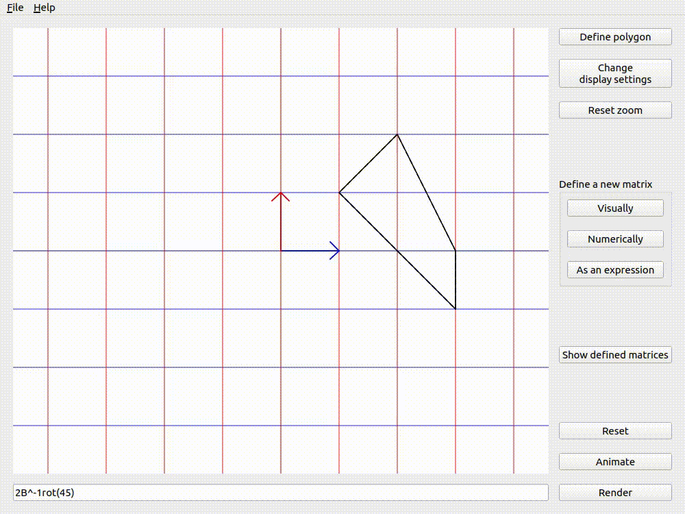
The version with the dashed outline is the untransformed version, whereas the one with the solid outline has been transformed by \(2\mathbf{B}^{-1}\mathbf{R}_{45}\).